Elements of Riemannian Geometry

Professor Dr. Arshad Momen

August 07, 2021

A geodesic is commonly a curve representing in some sense the shortest path between two points in a surface, or more generally in a Riemannian manifold

We saw that manifolds are sets whose subsets have a bijective mapping to subsets of $\mathbb{R}^n$. As there is a natural differentiable structure on $\mathbb{R}^n$ the manifold hence inherits a diffentiable structure on it too.

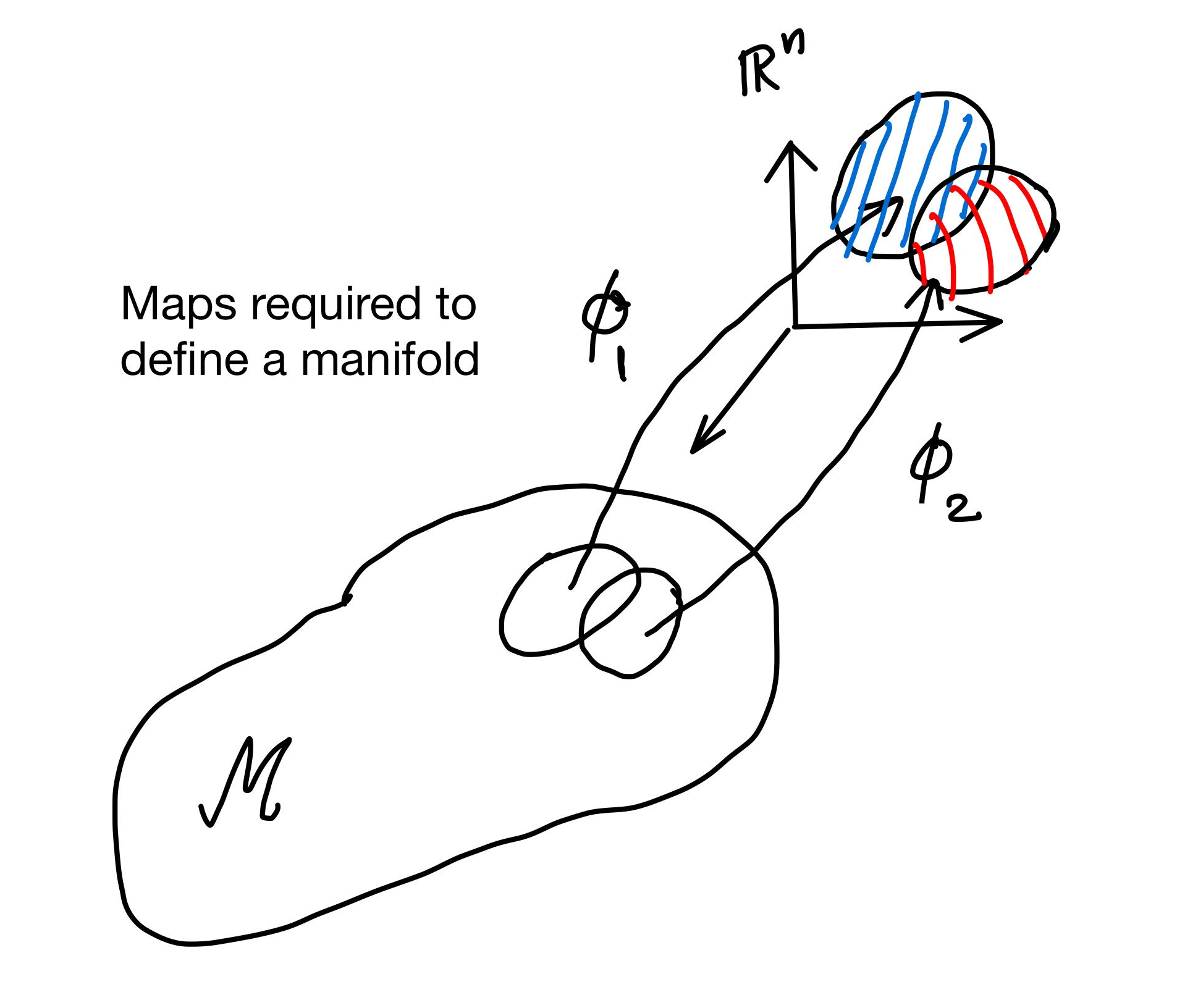
Figure: Map for Manifolds

Now now can thus import the concept of "distance" in $\mathbb{R}^n$ to the manifold $\mathcal{M}$ via the existence of this bijection.

The metric (which is a rank-2 symmetric tensor) is given by the existence of the symmetric form :

\begin{equation} ds^2 = g_{ij}(x) dx^i dx^j \Rightarrow (ds)^2=(d \pmb{x})^T G~ (d \pmb{x}) \end{equation}

where $G $ is a symmetric and invertible matrix representing the metric $g_{ij}$.

Let us consider a simple example:

In the first quadrant in the $xy$ plane we can introduce the coordinates $(u,v)$ :

\begin{equation} xy=u;~~ y=vx \Rightarrow x= \sqrt{\frac{u}{v}}, ~~~~ y= \sqrt{u v} \end{equation}

So that $ dx= \frac{1}{2} \sqrt{\frac{u}{v}}( \frac{du}{u} - \frac{dv}{v})$ and $dy = \sqrt{uv}( \frac{du}{u} + \frac{dv}{v})$

Plugging this back into $ds^2 = dx^2 + dy^2 $ and carrying out the standard algebra one ends up with the matrix for the

$$ G = \left( \begin{array}{ll} \frac{ \left(\sqrt{\frac{u}{v}}+\sqrt{u v}\right)}{u^2} & ~~\frac{ \left(\sqrt{u v}-\sqrt{\frac{u}{v}}\right)}{u v} \\ \frac{ \left(\sqrt{u v}-\sqrt{\frac{u}{v}}\right)}{u v} & ~~\frac{ \left(\sqrt{\frac{u}{v}}+\sqrt{u v}\right)}{v^2} \end{array} \right) $$

The presence of a metric thus allows us to define the arc length along a curve $\pmb{x} = \pmb{x}(\tau)$, where $\tau$ is the parameter along the arc:

\begin{equation} \int_A^B d\tau ~\sqrt{g_{ij}(\pmb{x}) \frac{d\pmb{x}^i}{d\tau} \frac{d\pmb{x}^j}{d\tau}} \label{length} \end{equation}

An interesting property to note that this expression is invariant under the reparameterization $\tau \rightarrow \tau'$ , establishing that we are indeed measuring something geometrical related to the curve.

The Geodesic

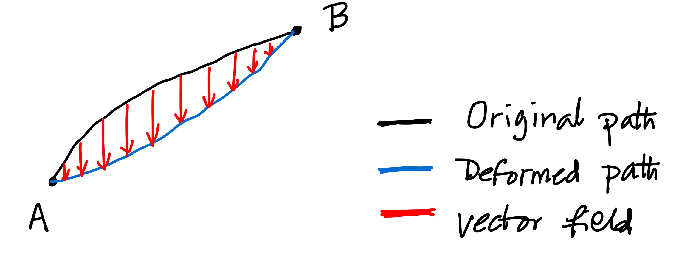
Our expression (\ref{length}) is valid for any curve. However if one is interested in the shortest curve ( which is known as geodesic) between two points, one has to minimize the expression (\ref{length}) under a local change

\begin{equation} \pmb{x} \rightarrow \pmb{x'} \equiv \pmb{x} +\delta \pmb{x} \label{varia} \end{equation}

in the function $\pmb{x} : \tau \rightarrow \mathbb{R}^n$. Note that

We can think of the variation, $\delta \pmb{x} = \pmb{x'} - \pmb{x} \equiv \epsilon ~\pmb{v}$ as a vector field defined over the curve in question.

The infinitesimal parameter $\epsilon$ is introduced just to emphasize that we will only keep terms first order in $\epsilon$ in our manipulations.

Let us rewrite (\ref{length}) as

\begin{equation} s = \int_A^B d\tau \sqrt{F}, \qquad ~~ F\equiv F[g, \pmb{x} ] = g_{ij}(\pmb{x}) \dot{x}^i \dot{x}^j \label{length2} \end{equation}

If $s $ is a local extrema ( just like 1D calculus ) its change under the change (\ref{varia}) will be zero: $ \delta s =0$. Thus

\begin{equation} \delta s = \frac{1}{2} \int d\tau~ \frac{1}{\sqrt{F}} \delta F =0 \label{vary} \end{equation}

Now this equation shows that if we extremize instead the functional:

$$ s'= \int_A^B d\tau ~F \Rightarrow \delta s' = \int_A^B d\tau ~\delta F $$

i.e. we will end up with the same local minima. One can see

$$ \delta F = \frac{\partial F}{\partial g_{ij}} \delta g_{ij}(\pmb{x}) + \frac{\partial F}{\partial \dot{x}^i} \delta \dot{x}^i = \dot{x}^i \dot{x}^j \delta g_{ij}(\pmb{x}) + 2 g_{ij}(\pmb{x}) \dot{x}^j \delta \dot{x}^i $$

Now some math gymnastics ( Sorry! Tokyo Olympics is on ):

$$ \delta \dot{x}^i = \frac{d}{d\tau} ( \delta x^i) \qquad \delta g_{ij} = \frac{\partial g_{ij}}{\partial x^k } \delta x^k $$

So that

$$ \delta s' = \int_A^B d\tau \left[ \dot{x}^i \dot{x}^j \frac{\partial g_{ij}}{\partial x^k } \delta x^k + 2 g_{kj} \dot{x}^j \frac{d}{d\tau} ( \delta x^k) \right] $$

The second term can be integrated by parts :

$$\delta s' = \int_A^B d\tau \left[ \dot{x}^i \dot{x}^j \frac{\partial g_{ij}}{\partial x^k } - 2 \frac{d}{d\tau}\left(g_{kj} \dot{x}^j \right)\right] \delta x^k $$

The "boundary" term vanishes as $\delta \pmb{x}$ vanish there.

So the geodesic equation can be obtained from the condition:

$$ \frac{d}{d\tau}\left(g_{kj} \dot{x}^j \right) - \frac{1}{2} \dot{x}^i \dot{x}^j \frac{\partial g_{ij}}{\partial x^k } = g_{jk} \ddot{x}^k + \frac{\partial g_{jk}}{\partial x^i} \dot{x}^i \dot{x}^j - \frac{1}{2} \dot{x}^i \dot{x}^j \frac{\partial g_{ij}}{\partial x^k } = 0 $$

As $\dot{x}^i \dot{x}^j $ is symmetric under the exchange of the indices $ i \leftrightarrow j$ we can rewrite the 2nd term

$$ \frac{\partial g_{jk}}{\partial x^i} \dot{x}^i \dot{x}^j = \frac{1}{2} \left( \frac{\partial g_{jk}}{\partial x^i} + \frac{\partial g_{ik}}{\partial x^j} \right)\dot{x}^i \dot{x}^j. $$

Putting all of these together

$$ g_{jk}( \pmb{x}) \ddot{x}^k + \frac{1}{2} \left[ \frac{\partial g_{jk}}{\partial x^i} + \frac{\partial g_{ik}}{\partial x^j} -\frac{\partial g_{ij}}{\partial x^k} \right] \dot{x}^i \dot{x}^j = 0. $$

As $G=\{g_{jk}\}$ is an invertible matrix, we can remove the $g_{jk}$ from the first term :

\begin{equation} \ddot{x}^m + \Gamma^m_{ij} \dot{x}^i \dot{x}^j =0 \end{equation}

where

$$ \Gamma^m_{ij} \equiv \frac{1}{2} g^{mk} \left[ \frac{\partial g_{jk}}{\partial x^i} + \frac{\partial g_{ik}}{\partial x^j} -\frac{\partial g_{ij}}{\partial x^k} \right] $$

which is known as Christoffel's (second) symbol. Despite carrying several indices it is not a tensor!

Note $g^{ij}$ are the matrix elements of the inverse $G^{-1}$.