Topics on Linear Algebra for Data Analysis - Part 2

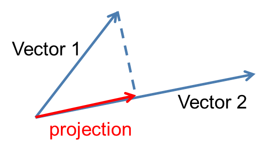Projection of a vector onto another vector has many important applications

Orthogonal Projection and Least Square Approximation

Orthogonal Projection: The Linear Algebra Way

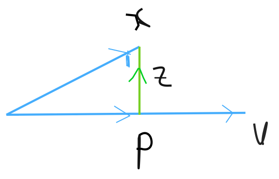
1. Projection on a vector: The orthogonal decomposition of $\boldsymbol{x}$ on $\boldsymbol{v}$ means

   $\boldsymbol{x}=\boldsymbol{p+z}$ such that $\boldsymbol{p}=t\boldsymbol{v}$ ($t$ is scalar) and $\boldsymbol{z}\perp \boldsymbol{v}$. $p = proj_\boldsymbol{v}x$ is called the orthogonal projection of $x$ on $v$. Show,

   $$\boldsymbol{p}=\frac{\boldsymbol{x^T v}}{\boldsymbol{v^T v}}\boldsymbol{v}$$

   and if $\boldsymbol{v}$ is an unit vector, then $\boldsymbol{p=(x^T v)v}$. Note that here we can consider $\boldsymbol{x^T v}$ as the coordinate of $\boldsymbol{p}$ in the space spanned by $\boldsymbol{p}$.

   
   
   Solution:
   

   Let $\boldsymbol{p}=t\boldsymbol{v}$, here t is a scalar

   $\boldsymbol{z}=\boldsymbol{x-p}=\boldsymbol{x}-t\boldsymbol{v}$

   $\boldsymbol{z}$ is orthogonal to $\boldsymbol{v}$ if and only if $$\mathbf{0}=(\boldsymbol{x}-t\boldsymbol{v}).\boldsymbol{v}$$ $$\Rightarrow \mathbf{0}=\boldsymbol{x.v}-(t\boldsymbol{v}.\boldsymbol{v})$$ $$\Rightarrow \boldsymbol{0}=\boldsymbol{x.v}-t(\boldsymbol{v.v})$$ $$\Rightarrow \boldsymbol{0}=\boldsymbol{x^T v}-t\boldsymbol{v^T v}$$ $$\therefore t= \frac{\boldsymbol{x^T v}}{\boldsymbol{v^T v}}$$ Since $\boldsymbol{p}=t\boldsymbol{v}$, we can write $$\boldsymbol{p}=\frac{\boldsymbol{x^T v}}{\boldsymbol{v^T v}}\boldsymbol{v}$$ If $\boldsymbol{v}$ is an unit vector, then $\boldsymbol{v.v}=1$ $$\therefore \boldsymbol{p=(x^T v)v}$$




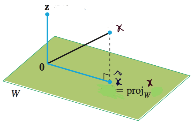
2. Projection on a subspace: Projection of $\boldsymbol{x}$ on a subspace $W$, such that $\boldsymbol{x}\notin \boldsymbol{W}$, is given by

   $$\boldsymbol{p}=proj_W \boldsymbol{x}=\hat{\boldsymbol{x}}=V V^T\boldsymbol{x}$$

   here, $\boldsymbol{W}$ is spanned by orthonormal basis set $B= \{v_1, v_2,\dots, v_k\}$ and
   $V = [v_1, v_2, \dots, v_k]$, the matrix with the $v_i$'s as columns.

   $VV^T$ is called the projection matrix.

   
   
   
   Solution: $\boldsymbol{x}=\boldsymbol{p+z}$ s.t., $\boldsymbol{p}\in\boldsymbol{W}$ or, $\hat{\boldsymbol{x}}\in\boldsymbol{W}$
   Then, $\hat{\boldsymbol{x}}=\boldsymbol{p}=\alpha_1 \boldsymbol{v_1}+..+\alpha_k \boldsymbol{v_k}=\boldsymbol{V}\boldsymbol{\alpha}$
   and $\boldsymbol{z} = \boldsymbol{x}-\boldsymbol{V\alpha}$ We also have, $\boldsymbol{z}\perp\boldsymbol{W}$ which means $\boldsymbol{z}\perp\boldsymbol{w}$, for any $\boldsymbol{w}\in\boldsymbol{W}$. Then $\boldsymbol{z}\perp\boldsymbol{v_i}$ because $\boldsymbol{z}$ is in $\boldsymbol{W}^{\perp}$ and subspace W is spanned by the orthonormal basis vectors $\boldsymbol{v_i}$.
   So, $$\boldsymbol{z}\perp\boldsymbol{v_1} \Rightarrow \boldsymbol{v_1^T z}=0\Rightarrow \boldsymbol{v_1^T}(\boldsymbol{x}-\boldsymbol{V\alpha})=0 $$ $$ \vdots$$ $$\boldsymbol{z}\perp\boldsymbol{v_k} \Rightarrow \boldsymbol{v_k^T z}=0\Rightarrow \boldsymbol{v_k^T}(\boldsymbol{x}-\boldsymbol{V\alpha})=0$$ Therefore, $$\begin{pmatrix} \boldsymbol{v_1^T}\\ \boldsymbol{v_2^{T}}\\ \vdots\\ \boldsymbol{v_k^{T}} \end{pmatrix}\boldsymbol{(}\boldsymbol{x}-\boldsymbol{V\alpha}\boldsymbol{)}=\boldsymbol{0}$$ $$\boldsymbol{V^T}\boldsymbol{(}\boldsymbol{x}-\boldsymbol{V\alpha}\boldsymbol{)}=\boldsymbol{0}$$ $$\Rightarrow \boldsymbol{V^T x}-\boldsymbol{V^T V\alpha}=\boldsymbol{0}$$ $$\Rightarrow \boldsymbol{V^T x}-\boldsymbol{\alpha}=\boldsymbol{0}$$ Since $\boldsymbol{V^T V}=\boldsymbol{I}$ ( Property of orthonormal matrix and here $\boldsymbol{V}$ is orthonormal matrix) $$\therefore \boldsymbol{\alpha}=\boldsymbol{V^T x}$$ We have $\hat{\boldsymbol{x}}=\boldsymbol{V \alpha}$ $$\therefore \hat{\boldsymbol{x}}=\boldsymbol{V V^T x}$$
   Note: Projection of $\boldsymbol{x}$ in the direction of $\boldsymbol{v_i}$, for $i=1,2, \dots,k$: $$proj_{\boldsymbol{v_i}}{\boldsymbol{x}}=(\boldsymbol{x^Tv_i)v_i}$$
   Therefore projection to the subspace can be expressed as $$ \begin{split} \hat{\boldsymbol{x}} & = proj_{W}{\boldsymbol{x}} = \boldsymbol{VV^T}\boldsymbol{x} \\ & =(\boldsymbol{x^Tv_1)v_1}+(\boldsymbol{x^Tv_2)v_2}+\dots+(\boldsymbol{x^Tv_k)v_k}\\ & = proj_{\boldsymbol{v_1}}\boldsymbol{x}+ proj_{\boldsymbol{v_2}}\boldsymbol{x}+\dots+proj_{\boldsymbol{v_k}}\boldsymbol{x} \end{split} $$


3. Orthogonal Projection Gives the Best Approximation: Using Pythagorean Theorem show that, $\left\|{\boldsymbol{x-p}}\right\|^2 < {\left\|\boldsymbol{x-q}\right\|}^2$, where $\boldsymbol{p} = proj_W \boldsymbol{x}$, $\boldsymbol{q}$ is in W, and $\boldsymbol{p}\neq \boldsymbol{q}$. That is, $\boldsymbol{p}$ is the best approximation of $\boldsymbol{x}$ in the subspace W. Solution:
   
   
   Both $\boldsymbol{p}$ and $\boldsymbol{q}$ are in $\boldsymbol{W}$ and distinct from each other. Then $\boldsymbol{p-q}$ is in $\boldsymbol{W}$. $\boldsymbol{z} = \boldsymbol{x-p}$ is orthogonal to $\boldsymbol{W}$. In particular, $\boldsymbol{x-p}$ is orthogonal to $\boldsymbol{p-q}$. Therefore, $$\boldsymbol{x-q}=(\boldsymbol{x-p})+(\boldsymbol{p-q})$$ Using Pythagorean Theorem, $$\left\|{\boldsymbol{x-q}}\right\|^2=\left\|{\boldsymbol{x-p}}\right\|^2+\left\|{\boldsymbol{p-q}}\right\|^2 $$ Now $\left\|{\boldsymbol{p-q}}\right\|^2>\boldsymbol{0}$ because $\boldsymbol{p-q}\neq \boldsymbol{0}$ which implies $\left\|{\boldsymbol{x-p}}\right\|^2<\left\|{\boldsymbol{x-q}}\right\|^2$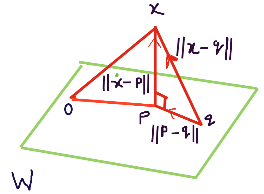


4. Change of Coordinates:
   $$ \begin{split} proj_W\boldsymbol{x} &= \boldsymbol{VV^Tx}\\ & = \begin{bmatrix} |& &|\\ \boldsymbol{v_1}&...&\boldsymbol{v_k}\\ |& &| \end{bmatrix} \begin{bmatrix} \boldsymbol{v_1^{T}}\\ \boldsymbol{v_2^{T}}\\ \vdots\\ \boldsymbol{v_k^{T}}\\ \end{bmatrix}\boldsymbol{x}\\ & = \begin{bmatrix} |& &|\\ \boldsymbol{v_1}& \dots &\boldsymbol{v_k}\\ |& &| \end{bmatrix}\begin{bmatrix} \boldsymbol{x^{T}v_1}\\ \boldsymbol{x^{T}v_2}\\ \vdots\\ \boldsymbol{x^{T}v_k} \end{bmatrix}\\ & = \begin{bmatrix} |& &|\\ \boldsymbol{v_1}& \dots &\boldsymbol{v_k}\\ |& &| \end{bmatrix}\begin{bmatrix} \alpha_{1}\\ \alpha_{2}\\ \vdots\\ \alpha_{k} \end{bmatrix}\\ &\therefore\big[\hat{\boldsymbol{x}}\big]_{S}=V \big[\hat{\boldsymbol{x}}\big]_{B} \end{split} $$
Observe that
1. $V^T \boldsymbol{x} = \big[\hat{\boldsymbol{x}}\big]_{B}$ gives the coordinates of the projection (using basis $B$) and
2. then the coordinates of the projection are changed from the basis $B$ to $S$ (the standard basis).
3. $\big[\hat{\boldsymbol{x}}\big]_{S}$ is a $d{\times}1$ vector and $\big[\hat{\boldsymbol{x}}\big]_{B}$ is a $k{\times}1$ vector. If $\boldsymbol{x}$ is from a $d$-dimensional vector space,

Orthogonal Projection: The Calculus Way

1. Projection on a vector: Using Calculus find the vector closest (in least square sense) to $\boldsymbol{x}$ in the direction of $\boldsymbol{v}$. In other words, find the least square approximation of $\boldsymbol{x}$ in the space spanned by $\boldsymbol{v}$.
   Solution: A vector $\boldsymbol{p}$ in the direction of $\boldsymbol{v}$ is given by $\boldsymbol{p}=t\boldsymbol{v}$, where $t$ is a scalar. Therefore, we need to find $t$ that minimizes $J(t)=\left\|{\boldsymbol{x}-t\boldsymbol{v}}\right\|^2$ $$J(t)=\left\|{\boldsymbol{x}-t\boldsymbol{v}}\right\|^2$$ $$\Rightarrow J(t)= (\boldsymbol{x}-t\boldsymbol{v})^T (\boldsymbol{x}-t\boldsymbol{v})=(\boldsymbol{x}^T-t\boldsymbol{v}^T)(\boldsymbol{x}-t\boldsymbol{v})$$ $$\Rightarrow J(t)=\boldsymbol{x}^T\boldsymbol{x}-t\boldsymbol{v}^T\boldsymbol{x} - t\boldsymbol{x}^T\boldsymbol{v}+t^2(\boldsymbol{v}^T\boldsymbol{v})$$ $$\begin{equation} \label{firsteq} \therefore J(t)=\left\|{\boldsymbol{x}}\right\|^2-2t\boldsymbol{x}^T\boldsymbol{v}+t^2\left\|{\boldsymbol{v}}\right\|^2 \end{equation}$$ Differentiating equation (\ref{firsteq}) with respect to $t$, we get, $$J'(t)=-2\boldsymbol{x}^T\boldsymbol{x}+2t\left\|{\boldsymbol{v}}\right\|^2$$ Setting $J'(t)=0$ and solving for $t$ we get, $$-2\boldsymbol{x}^T\boldsymbol{v}+2t\left\|{\boldsymbol{v}}\right\|^2=0$$ $$\therefore t=\frac{\boldsymbol{x}^T\boldsymbol{v}}{\left\|{\boldsymbol{v}}\right\|^2}$$ Therefore, projection of $\boldsymbol{x}$ on $\boldsymbol{v}$ defined as $\boldsymbol{p}$ can be written as, $$\boldsymbol{p}=\frac{\boldsymbol{x}^T \boldsymbol{v}}{\left\|{\boldsymbol{v}}\right\|^2}\boldsymbol{v}$$


2. Projection on a subspace: We seek the closest approximation of vector $\boldsymbol{x}$ in the subspace $\boldsymbol{W}$ which has dimension $k$. Assume, $\boldsymbol{v_i}$'s for $i=1,2,...,k$ form an orthonormal basis for $\boldsymbol{W}$. Find the $\alpha_{i}$'s for $i=1,2,...,k$, s.t. the error $J$, given by %$\boldsymbol{\alpha_1,...,\alpha_N}$ \[ J = \big\|{\boldsymbol{x-\hat{\boldsymbol{x}}}}\big\|^{2} = \big\|{\boldsymbol{x}-\sum_{i=1}^{k}\alpha_{i}\boldsymbol{v}_i}\big\| ^{2}\] is minimized.
   Solution: Any vector in $\boldsymbol{W}$ can be written as $\sum_{i=1}^{k}\alpha_i\boldsymbol{v}_i$. Thus, $\boldsymbol{x}$ will be represented by some vector in $\boldsymbol{W}$ as $\sum_{i=1}^{k}\alpha_i\boldsymbol{v}_i$. To minimize the error J we need to take partial derivatives. $$ \begin{equation} \begin{split} J(\alpha_{1},...,\alpha_{k})&= \big\|{\boldsymbol{x}-\sum_{i=1}^{k}\alpha_{i}\boldsymbol{v}_i}\big\|^{2} \\ &= (\boldsymbol{x}-\sum_{i=1}^{k} \alpha_i\boldsymbol{v}_i)^T (\boldsymbol{x} - \sum_{i=1}^{k}\alpha_i\boldsymbol{v}_i)\\ &= (\boldsymbol{x}^T-\sum_{i=1}^{k} \alpha_{i}\boldsymbol{v}_i^T) (\boldsymbol{x}-\sum_{i=1}^{k}\alpha_i\boldsymbol{v}_i)\\ &= \boldsymbol{x}^T \boldsymbol{x}-\boldsymbol{x}\sum_{i=1}^{k} \alpha_{i}\boldsymbol{v}_i^T -\boldsymbol{x}^T\sum_{i=1}^{k}\alpha_{i \boldsymbol{v}_i}+(\sum_{i=1}^{k}\alpha_i\boldsymbol{v}_i^T) (\sum_{i=1}^{k}\alpha_i \boldsymbol{v}_i)\\ &=\big\|\boldsymbol{x}\big\|^2-2\sum_{i=1}^{k}\alpha_i \boldsymbol{x}^T\boldsymbol{v}_i +\sum_{i=1}^{k}\alpha_i ^2 \Bigg[\because \big\|\boldsymbol{v}_i\big\|^2=1 \text{ and } \boldsymbol{v}_i\text{'s are orthogonal}\Bigg] \end{split} \end{equation} $$
   Then we take partial derivative with respect to $\alpha_{i}$ and set that to 0 for optimal value. We get, $$-2\boldsymbol{x}^T\boldsymbol{v}_{i}+2\alpha_{i}= 0$$ $$\therefore \alpha_i =\boldsymbol{x}^T\boldsymbol{v}_i$$

Ordinary Least Square Regression

Suppose we have $N$ datapoints $(\boldsymbol{x}^{(1)}, y^{(1)}), \ldots , (\boldsymbol{x}^{(N)}, y^{(N)})$, where $\boldsymbol{x}^{(i)}$'s are $d$-vectors $[\boldsymbol{x}^{(i)}_1, \boldsymbol{x}^{(i)}_2, \dots, \boldsymbol{x}^{(i)}_d]$ (\textit{i.e., $x$ contains the values of $d$ features or (independent) variables}) and $y$ is a real number (\textit{called the dependent variable}).

We assume there is a function $f(\boldsymbol{x})$ such that $y = f(\boldsymbol{x})$. In linear regression, based on the data, we want to find a linear (affine) function $\hat{f}$ that approximates $f$(in the least square sense).

Let,

That means, we need to find the $\beta_0, ..., \beta_d$ coefficinets that satisfy the above equations. We can view this problem as finding the solution to the system of linear equations ($\boldsymbol{A} \boldsymbol{\beta} = \mathbf{\hat{y}}$). However, this is a overdetermined system (more equations (or rows) than variables (or columns)). Therefore, we can only find the best $\boldsymbol{\beta}$ that approximately solves the system of linear equation.

Or, we can also view this as an optimization problem and find the $\boldsymbol{\beta}$ that minimizes the Mean Squared Error (MSE):

Note: Usually in linear regression the features or independent variables are transformed to create a new set of variables. This can be done through basis functions $\phi_j(\mathbf{x})$ that transforms the data and creates a datapoint in the transformed feature space, $z_j = \phi_j(\mathbf{x}), \; \; j = 1, \ldots ,p$. And then we do linear regression using the transformed datapoints, Note that The basis functions can be non-linear.

Again, the MSE can be written as

where,

The Linear Algebra Way

Suppose we have a system of linear equations $A\boldsymbol{\beta}=\boldsymbol{y}$, where $A$ is a $N \times k$ matrix.

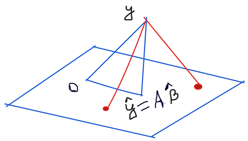
If the system of linear equations does not have a solution, $\boldsymbol{y} \neq \beta_1\boldsymbol{a_1}+ \beta_2\boldsymbol{a_2}+\dots+\beta_k\boldsymbol{a_k}$, i.e., $\boldsymbol{y} \notin Col(A)=span\{\boldsymbol{a_1}, \boldsymbol{a_2}, \dots \boldsymbol{a_k}\}$. Then least square solution is $\hat{\boldsymbol{\beta}}$, such that $\left\|{\boldsymbol{y}-A\boldsymbol{\hat{\boldsymbol{\beta}}}}\right\|^2$ is minimum.

We observe, what we are asking for is the coordinates of $\hat{y}=proj_{Col(A)}y$. Now, we may not have an orthonormal basis of $Col(A)$, that is columns of $A$ might not be orthonormal. Rather we have a basis $B'=\{\boldsymbol{a_1},\boldsymbol{a_2},...,\boldsymbol{a_k}\}$ of the $Col(A)$, assuming the columns of $A$ are linearly independent. Show, $$\hat{\boldsymbol{\beta}}=(A^T A)^{-1}A^T \boldsymbol{y}$$ $$\hat{\boldsymbol{y}}=proj_{Col(A)}\boldsymbol{y}=A\hat{\boldsymbol{\beta}}=A(A^T A)^{-1}A^T \boldsymbol{y}$$ Note, $A(A^T A)^{-1}A^T$ is called the Projection matrix and $A^\dagger=(A^T A)^{-1}A^T$ is called the pseudo-inverse matrix.

Solution: When a solution is demanded and none exists, in this scenario what we can do is to find a $\boldsymbol{\beta}$ that makes $A\boldsymbol{\beta}$ as close as possible to $\boldsymbol{y}$. Here, $A$ is $N \times k$ and $\boldsymbol{y}$ is in $\mathbb{R}^N$.

Let $\hat{\boldsymbol{y}}=$proj$_{Col(A)}\boldsymbol{y}$ Because $\hat{\boldsymbol{y}}$ is in the column space of $A$, the equation $A\boldsymbol{\beta}=\hat{\boldsymbol{y}}$ is consistent and there is a $\hat{\boldsymbol{\beta}}$ in $\mathbb{R}^k$ such that $$A\hat{\boldsymbol{\beta}}=\hat{\boldsymbol{y}}$$ The projection $\hat{\boldsymbol{y}}$ has the property that $\boldsymbol{y}-\hat{\boldsymbol{y}}$ is orthogonal to $Col(A)$, so $(\boldsymbol{y}-A\hat{\boldsymbol{\beta}})$ is orthogonal to each column of $A$. If $\boldsymbol{a_{j}}$ is any column of $A$, then $\boldsymbol{a_{j}.(y-}A\hat{\boldsymbol{\beta}})=\boldsymbol{0}$ and $\boldsymbol{a_{j}^T(y-}A\hat{\boldsymbol{\beta}})=\boldsymbol{0}$. Since each $\boldsymbol{a_{j}^T}$ is a row of $A^T$, $A^T(\boldsymbol{y}-A\hat{\boldsymbol{\beta}})=\boldsymbol{0}$ $\Rightarrow A^T\boldsymbol{y}-A^TA\hat{\boldsymbol{\beta}}=\boldsymbol{0}$ $\Rightarrow A^TA\hat{\boldsymbol{\beta}}=A^T\boldsymbol{y}$ [These are called the Normal Equations] $\therefore \hat{\boldsymbol{\beta}}=(A^T A)^{-1}A^T \boldsymbol{y}$ Finally we have, $\hat{\boldsymbol{y}}=$ proj$_\boldsymbol{Col(A)}\boldsymbol{y}=A\boldsymbol{\beta}=A(A^T A)^{-1}A^T \boldsymbol{y}$

Using QR decomposition:

Alternatively, $\hat{\boldsymbol{y}}=\boldsymbol{QQ^T}\boldsymbol{y}$ where A$=\boldsymbol{QR}$ is the $QR$ decomposition of $A$.

Here, the columns of $\boldsymbol{Q}$ form an orthonormal basis for $Col(A)$ and $\boldsymbol{R}$ is an upper triangular invertible matrix.

The Calculus Way

Using the derivative rules, we can use calculus to find the $\boldsymbol{\beta}$: